Get Started in 10 Minutes

Altay Sansal

Oct 20, 2025

9 min read

In this page we will be showing basic capabilities of MDIO.

For demonstration purposes, we will ingest the remote Teapot Dome open-source dataset. The dataset details and licensing can be found at the SEG Wiki.

We are using the 3D seismic stack dataset named filt_mig.sgy.

The full HTTP link for the dataset (hosted on AWS): http://s3.amazonaws.com/teapot/filt_mig.sgy

Warning

For plotting and remote ingestion the notebook requires Matplotlib and aiohttp as a dependency. Please install it before executing using pip install matplotlib aiohttp or conda install matplotlib aiohttp.

Defining the SEG-Y Dataset

Since MDIO 0.8 we can directly ingest remote SEG-Y files! The file is 386 MB in size. To make the header scan performant we can also set up an environment variable for MDIO. See here for when to use this: Buffered Reads in Ingestion.

The dataset is irregularly shaped, however it is padded to a rectangle with zeros (dead traces). We will see that later at the live mask plotting.

The following environment variables are essential here:

• MDIO__IMPORT__CLOUD_NATIVE tells MDIO to do buffered reads for headers due to remote file.

• MDIO__IMPORT__SAVE_SEGY_FILE_HEADER makes MDIO save the SEG-Y specific file headers (text, binary) which is not strictly necessary for consumption and is disabled by default.

import os

os.environ["MDIO__IMPORT__CLOUD_NATIVE"] = "true"
os.environ["MDIO__IMPORT__SAVE_SEGY_FILE_HEADER"] = "true"

input_url = "http://s3.amazonaws.com/teapot/filt_mig.sgy"

Ingesting to MDIO

To do this, we can use the convenient SEG-Y to MDIO converter.

The inline and crossline values are located at bytes 181 and 185. Note that this doesn’t match any SEG-Y standards.

MDIO uses TGSAI/segy to parse the SEG-Y; the field names conform to its canonical keys defined in SEGY Binary Header Keys and SEGY Trace Header Keys. Since MDIO v1 we also introduced templates for common seismic data types. For instance, we will be using the PostStack3DTime template here, which expects the same canonical keys.

We will also specify the units for the time domain. The spatial units will be automatically parsed from SEG-Y binary header. However, there may be a case where it is corrupt in the file, for that see the Fixing X/Y Units Issues section.

In summary, we will use the byte locations as defined for ingestion.

import matplotlib.pyplot as plt
from segy.schema import HeaderField
from segy.standards import get_segy_standard

from mdio import segy_to_mdio
from mdio.builder.schemas.v1.units import TimeUnitModel
from mdio.builder.template_registry import get_template

teapot_trace_headers = [
    HeaderField(name="inline", byte=181, format="int32"),
    HeaderField(name="crossline", byte=185, format="int32"),
    HeaderField(name="cdp_x", byte=189, format="int32"),
    HeaderField(name="cdp_y", byte=193, format="int32"),
]

rev0_segy_spec = get_segy_standard(0)
teapot_segy_spec = rev0_segy_spec.customize(trace_header_fields=teapot_trace_headers)

mdio_template = get_template("PostStack3DTime")
unit_ms = TimeUnitModel(time="ms")
mdio_template.add_units({"time": unit_ms})

segy_to_mdio(
    input_path=input_url,
    output_path="filt_mig.mdio",
    segy_spec=teapot_segy_spec,
    mdio_template=mdio_template,
    overwrite=True,
)

It only took a few seconds to ingest, since this is a very small file.

However, MDIO scales up to TB (that’s ~1,000 GB) sized volumes!

Opening the Ingested MDIO File

Let’s open the MDIO file with the open_mdio function. This will return a pretty xarray representation with our standardized format.

from mdio import open_mdio

dataset = open_mdio("filt_mig.mdio")
dataset

<xarray.Dataset> Size: 403MB
Dimensions:           (inline: 345, crossline: 188, time: 1501)
Coordinates:
  * inline            (inline) int32 1kB 1 2 3 4 5 6 ... 340 341 342 343 344 345
  * crossline         (crossline) int32 752B 1 2 3 4 5 6 ... 184 185 186 187 188
  * time              (time) int32 6kB 0 2 4 6 8 10 ... 2992 2994 2996 2998 3000
    cdp_y             (inline, crossline) float64 519kB ...
    cdp_x             (inline, crossline) float64 519kB ...
Data variables:
    trace_mask        (inline, crossline) bool 65kB ...
    segy_file_header  <U1 4B ...
    amplitude         (inline, crossline, time) float32 389MB ...
    headers           (inline, crossline) [('trace_seq_num_line', '<i4'), ('trace_seq_num_reel', '<i4'), ('orig_field_record_num', '<i4'), ('trace_num_orig_record', '<i4'), ('energy_source_point_num', '<i4'), ('ensemble_num', '<i4'), ('trace_num_ensemble', '<i4'), ('trace_id_code', '<i2'), ('vertically_summed_traces', '<i2'), ('horizontally_stacked_traces', '<i2'), ('data_use', '<i2'), ('source_to_receiver_distance', '<i4'), ('receiver_group_elevation', '<i4'), ('source_surface_elevation', '<i4'), ('source_depth_below_surface', '<i4'), ('receiver_datum_elevation', '<i4'), ('source_datum_elevation', '<i4'), ('source_water_depth', '<i4'), ('receiver_water_depth', '<i4'), ('elevation_depth_scalar', '<i2'), ('coordinate_scalar', '<i2'), ('source_coord_x', '<i4'), ('source_coord_y', '<i4'), ('group_coord_x', '<i4'), ('group_coord_y', '<i4'), ('coordinate_unit', '<i2'), ('weathering_velocity', '<i2'), ('subweathering_velocity', '<i2'), ('source_uphole_time', '<i2'), ('group_uphole_time', '<i2'), ('source_static_correction', '<i2'), ('receiver_static_correction', '<i2'), ('total_static_applied', '<i2'), ('lag_time_a', '<i2'), ('lag_time_b', '<i2'), ('delay_recording_time', '<i2'), ('mute_time_start', '<i2'), ('mute_time_end', '<i2'), ('samples_per_trace', '<i2'), ('sample_interval', '<i2'), ('instrument_gain_type', '<i2'), ('instrument_gain_const', '<i2'), ('instrument_gain_initial', '<i2'), ('correlated_data', '<i2'), ('sweep_freq_start', '<i2'), ('sweep_freq_end', '<i2'), ('sweep_length', '<i2'), ('sweep_type', '<i2'), ('sweep_taper_start', '<i2'), ('sweep_taper_end', '<i2'), ('taper_type', '<i2'), ('alias_filter_freq', '<i2'), ('alias_filter_slope', '<i2'), ('notch_filter_freq', '<i2'), ('notch_filter_slope', '<i2'), ('low_cut_freq', '<i2'), ('high_cut_freq', '<i2'), ('low_cut_slope', '<i2'), ('high_cut_slope', '<i2'), ('year_recorded', '<i2'), ('day_of_year', '<i2'), ('hour_of_day', '<i2'), ('minute_of_hour', '<i2'), ('second_of_minute', '<i2'), ('time_basis_code', '<i2'), ('trace_weighting_factor', '<i2'), ('group_num_roll_switch', '<i2'), ('group_num_first_trace', '<i2'), ('group_num_last_trace', '<i2'), ('gap_size', '<i2'), ('taper_overtravel', '<i2'), ('inline', '<i4'), ('crossline', '<i4'), ('cdp_x', '<i4'), ('cdp_y', '<i4')] 13MB ...
Attributes:
    apiVersion:  1.0.8
    createdOn:   2025-10-20 15:52:03.112832+00:00
    name:        PostStack3DTime
    attributes:  {'surveyType': '3D', 'gatherType': 'stacked', 'defaultVariab...

xarray.Dataset

• Dimensions:
  • inline: 345
  • crossline: 188
  • time: 1501
• Coordinates: (5)
  • inline
    (inline)
    int32
    1 2 3 4 5 6 ... 341 342 343 344 345

    array([  1,   2,   3, ..., 343, 344, 345], shape=(345,), dtype=int32)

  • crossline
    (crossline)
    int32
    1 2 3 4 5 6 ... 184 185 186 187 188

    array([  1,   2,   3,   4,   5,   6,   7,   8,   9,  10,  11,  12,  13,  14,
            15,  16,  17,  18,  19,  20,  21,  22,  23,  24,  25,  26,  27,  28,
            29,  30,  31,  32,  33,  34,  35,  36,  37,  38,  39,  40,  41,  42,
            43,  44,  45,  46,  47,  48,  49,  50,  51,  52,  53,  54,  55,  56,
            57,  58,  59,  60,  61,  62,  63,  64,  65,  66,  67,  68,  69,  70,
            71,  72,  73,  74,  75,  76,  77,  78,  79,  80,  81,  82,  83,  84,
            85,  86,  87,  88,  89,  90,  91,  92,  93,  94,  95,  96,  97,  98,
            99, 100, 101, 102, 103, 104, 105, 106, 107, 108, 109, 110, 111, 112,
           113, 114, 115, 116, 117, 118, 119, 120, 121, 122, 123, 124, 125, 126,
           127, 128, 129, 130, 131, 132, 133, 134, 135, 136, 137, 138, 139, 140,
           141, 142, 143, 144, 145, 146, 147, 148, 149, 150, 151, 152, 153, 154,
           155, 156, 157, 158, 159, 160, 161, 162, 163, 164, 165, 166, 167, 168,
           169, 170, 171, 172, 173, 174, 175, 176, 177, 178, 179, 180, 181, 182,
           183, 184, 185, 186, 187, 188], dtype=int32)

  • time
    (time)
    int32
    0 2 4 6 8 ... 2994 2996 2998 3000

    unitsV1 :

    {'time': 'ms'}

    array([   0,    2,    4, ..., 2996, 2998, 3000], shape=(1501,), dtype=int32)

  • cdp_y
    (inline, crossline)
    float64
    ...

    unitsV1 :

    {'length': 'ft'}

    [64860 values with dtype=float64]

  • cdp_x
    (inline, crossline)
    float64
    ...

    unitsV1 :

    {'length': 'ft'}

    [64860 values with dtype=float64]

• Data variables: (4)
  • trace_mask
    (inline, crossline)
    bool
    ...

    [64860 values with dtype=bool]

  • segy_file_header
    ()
    <U1
    ...

    textHeader :

    C 1 CLIENT: ROCKY MOUNTAIN OILFIELD TESTING CENTER C 2 PROJECT: NAVAL PETROLEUM RESERVE #3 (TEAPOT DOME); NATRONA COUNTY, WYOMING C 3 LINE: 3D C 4 C 5 THIS IS THE FILTERED POST STACK MIGRATION C 6 C 7 INLINE 1, XLINE 1: X COORDINATE: 788937 Y COORDINATE: 938845 C 8 INLINE 1, XLINE 188: X COORDINATE: 809501 Y COORDINATE: 939333 C 9 INLINE 188, XLINE 1: X COORDINATE: 788039 Y COORDINATE: 976674 C10 INLINE NUMBER: MIN: 1 MAX: 345 TOTAL: 345 C11 CROSSLINE NUMBER: MIN: 1 MAX: 188 TOTAL: 188 C12 TOTAL NUMBER OF CDPS: 64860 BIN DIMENSION: 110' X 110' C13 C14 C15 C16 C17 C18 C19 GENERAL SEGY INFORMATION C20 RECORD LENGHT (MS): 3000 C21 SAMPLE RATE (MS): 2.0 C22 DATA FORMAT: 4 BYTE IBM FLOATING POINT C23 BYTES 13- 16: CROSSLINE NUMBER (TRACE) C24 BYTES 17- 20: INLINE NUMBER (LINE) C25 BYTES 81- 84: CDP_X COORD C26 BYTES 85- 88: CDP_Y COORD C27 BYTES 181-184: INLINE NUMBER (LINE) C28 BYTES 185-188: CROSSLINE NUMBER (TRACE) C29 BYTES 189-192: CDP_X COORD C30 BYTES 193-196: CDP_Y COORD C31 C32 C33 C34 C35 C36 Processed by: Excel Geophysical Services, Inc. C37 8301 East Prentice Ave. Ste. 402 C38 Englewood, Colorado 80111 C39 (voice) 303.694.9629 (fax) 303.771.1646 C40 END EBCDIC

    binaryHeader :

    {'job_id': 9999, 'line_num': 9999, 'reel_num': 1, 'data_traces_per_ensemble': 188, 'aux_traces_per_ensemble': 0, 'sample_interval': 2000, 'orig_sample_interval': 0, 'samples_per_trace': 1501, 'orig_samples_per_trace': 1501, 'data_sample_format': 1, 'ensemble_fold': 57, 'trace_sorting_code': 4, 'vertical_sum_code': 1, 'sweep_freq_start': 0, 'sweep_freq_end': 0, 'sweep_length': 0, 'sweep_type_code': 0, 'sweep_trace_num': 0, 'sweep_taper_start': 0, 'sweep_taper_end': 0, 'taper_type_code': 0, 'correlated_data_code': 2, 'binary_gain_code': 1, 'amp_recovery_code': 4, 'measurement_system_code': 2, 'impulse_polarity_code': 1, 'vibratory_polarity_code': 0, 'segy_revision_major': 0, 'segy_revision_minor': 0}

    [1 values with dtype=<U1]

  • amplitude
    (inline, crossline, time)
    float32
    ...

    statsV1 :

    {"count":46854270,"sum":-8594.551589292674,"sumSquares":40571285.423519716,"min":-8.375323295593262,"max":7.723702430725098,"histogram":{"counts":[],"binCenters":[]}}

    [97354860 values with dtype=float32]

  • headers
    (inline, crossline)
    [('trace_seq_num_line', '<i4'), ('trace_seq_num_reel', '<i4'), ('orig_field_record_num', '<i4'), ('trace_num_orig_record', '<i4'), ('energy_source_point_num', '<i4'), ('ensemble_num', '<i4'), ('trace_num_ensemble', '<i4'), ('trace_id_code', '<i2'), ('vertically_summed_traces', '<i2'), ('horizontally_stacked_traces', '<i2'), ('data_use', '<i2'), ('source_to_receiver_distance', '<i4'), ('receiver_group_elevation', '<i4'), ('source_surface_elevation', '<i4'), ('source_depth_below_surface', '<i4'), ('receiver_datum_elevation', '<i4'), ('source_datum_elevation', '<i4'), ('source_water_depth', '<i4'), ('receiver_water_depth', '<i4'), ('elevation_depth_scalar', '<i2'), ('coordinate_scalar', '<i2'), ('source_coord_x', '<i4'), ('source_coord_y', '<i4'), ('group_coord_x', '<i4'), ('group_coord_y', '<i4'), ('coordinate_unit', '<i2'), ('weathering_velocity', '<i2'), ('subweathering_velocity', '<i2'), ('source_uphole_time', '<i2'), ('group_uphole_time', '<i2'), ('source_static_correction', '<i2'), ('receiver_static_correction', '<i2'), ('total_static_applied', '<i2'), ('lag_time_a', '<i2'), ('lag_time_b', '<i2'), ('delay_recording_time', '<i2'), ('mute_time_start', '<i2'), ('mute_time_end', '<i2'), ('samples_per_trace', '<i2'), ('sample_interval', '<i2'), ('instrument_gain_type', '<i2'), ('instrument_gain_const', '<i2'), ('instrument_gain_initial', '<i2'), ('correlated_data', '<i2'), ('sweep_freq_start', '<i2'), ('sweep_freq_end', '<i2'), ('sweep_length', '<i2'), ('sweep_type', '<i2'), ('sweep_taper_start', '<i2'), ('sweep_taper_end', '<i2'), ('taper_type', '<i2'), ('alias_filter_freq', '<i2'), ('alias_filter_slope', '<i2'), ('notch_filter_freq', '<i2'), ('notch_filter_slope', '<i2'), ('low_cut_freq', '<i2'), ('high_cut_freq', '<i2'), ('low_cut_slope', '<i2'), ('high_cut_slope', '<i2'), ('year_recorded', '<i2'), ('day_of_year', '<i2'), ('hour_of_day', '<i2'), ('minute_of_hour', '<i2'), ('second_of_minute', '<i2'), ('time_basis_code', '<i2'), ('trace_weighting_factor', '<i2'), ('group_num_roll_switch', '<i2'), ('group_num_first_trace', '<i2'), ('group_num_last_trace', '<i2'), ('gap_size', '<i2'), ('taper_overtravel', '<i2'), ('inline', '<i4'), ('crossline', '<i4'), ('cdp_x', '<i4'), ('cdp_y', '<i4')]
    ...

    [64860 values with dtype=[('trace_seq_num_line', '<i4'), ('trace_seq_num_reel', '<i4'), ('orig_field_record_num', '<i4'), ('trace_num_orig_record', '<i4'), ('energy_source_point_num', '<i4'), ('ensemble_num', '<i4'), ('trace_num_ensemble', '<i4'), ('trace_id_code', '<i2'), ('vertically_summed_traces', '<i2'), ('horizontally_stacked_traces', '<i2'), ('data_use', '<i2'), ('source_to_receiver_distance', '<i4'), ('receiver_group_elevation', '<i4'), ('source_surface_elevation', '<i4'), ('source_depth_below_surface', '<i4'), ('receiver_datum_elevation', '<i4'), ('source_datum_elevation', '<i4'), ('source_water_depth', '<i4'), ('receiver_water_depth', '<i4'), ('elevation_depth_scalar', '<i2'), ('coordinate_scalar', '<i2'), ('source_coord_x', '<i4'), ('source_coord_y', '<i4'), ('group_coord_x', '<i4'), ('group_coord_y', '<i4'), ('coordinate_unit', '<i2'), ('weathering_velocity', '<i2'), ('subweathering_velocity', '<i2'), ('source_uphole_time', '<i2'), ('group_uphole_time', '<i2'), ('source_static_correction', '<i2'), ('receiver_static_correction', '<i2'), ('total_static_applied', '<i2'), ('lag_time_a', '<i2'), ('lag_time_b', '<i2'), ('delay_recording_time', '<i2'), ('mute_time_start', '<i2'), ('mute_time_end', '<i2'), ('samples_per_trace', '<i2'), ('sample_interval', '<i2'), ('instrument_gain_type', '<i2'), ('instrument_gain_const', '<i2'), ('instrument_gain_initial', '<i2'), ('correlated_data', '<i2'), ('sweep_freq_start', '<i2'), ('sweep_freq_end', '<i2'), ('sweep_length', '<i2'), ('sweep_type', '<i2'), ('sweep_taper_start', '<i2'), ('sweep_taper_end', '<i2'), ('taper_type', '<i2'), ('alias_filter_freq', '<i2'), ('alias_filter_slope', '<i2'), ('notch_filter_freq', '<i2'), ('notch_filter_slope', '<i2'), ('low_cut_freq', '<i2'), ('high_cut_freq', '<i2'), ('low_cut_slope', '<i2'), ('high_cut_slope', '<i2'), ('year_recorded', '<i2'), ('day_of_year', '<i2'), ('hour_of_day', '<i2'), ('minute_of_hour', '<i2'), ('second_of_minute', '<i2'), ('time_basis_code', '<i2'), ('trace_weighting_factor', '<i2'), ('group_num_roll_switch', '<i2'), ('group_num_first_trace', '<i2'), ('group_num_last_trace', '<i2'), ('gap_size', '<i2'), ('taper_overtravel', '<i2'), ('inline', '<i4'), ('crossline', '<i4'), ('cdp_x', '<i4'), ('cdp_y', '<i4')]]

• Attributes: (4)

  apiVersion :

  1.0.8

  createdOn :

  2025-10-20 15:52:03.112832+00:00

  name :

  PostStack3DTime

  attributes :

  {'surveyType': '3D', 'gatherType': 'stacked', 'defaultVariableName': 'amplitude'}

Querying Metadata

Now let’s look at the file text header saved in the segy_file_header metadata variable.

print(dataset["segy_file_header"].attrs["textHeader"])

C 1 CLIENT: ROCKY MOUNTAIN OILFIELD TESTING CENTER                              
C 2 PROJECT: NAVAL PETROLEUM RESERVE #3 (TEAPOT DOME); NATRONA COUNTY, WYOMING  
C 3 LINE: 3D                                                                    
C 4                                                                             
C 5 THIS IS THE FILTERED POST STACK MIGRATION                                   
C 6                                                                             
C 7 INLINE 1, XLINE 1:   X COORDINATE: 788937  Y COORDINATE: 938845             
C 8 INLINE 1, XLINE 188: X COORDINATE: 809501  Y COORDINATE: 939333             
C 9 INLINE 188, XLINE 1: X COORDINATE: 788039  Y COORDINATE: 976674             
C10 INLINE NUMBER:    MIN: 1  MAX: 345  TOTAL: 345                              
C11 CROSSLINE NUMBER: MIN: 1  MAX: 188  TOTAL: 188                              
C12 TOTAL NUMBER OF CDPS: 64860   BIN DIMENSION: 110' X 110'                    
C13                                                                             
C14                                                                             
C15                                                                             
C16                                                                             
C17                                                                             
C18                                                                             
C19 GENERAL SEGY INFORMATION                                                    
C20 RECORD LENGHT (MS): 3000                                                    
C21 SAMPLE RATE (MS): 2.0                                                       
C22 DATA FORMAT: 4 BYTE IBM FLOATING POINT                                      
C23 BYTES  13- 16: CROSSLINE NUMBER (TRACE)                                     
C24 BYTES  17- 20: INLINE NUMBER (LINE)                                         
C25 BYTES  81- 84: CDP_X COORD                                                  
C26 BYTES  85- 88: CDP_Y COORD                                                  
C27 BYTES 181-184: INLINE NUMBER (LINE)                                         
C28 BYTES 185-188: CROSSLINE NUMBER (TRACE)                                     
C29 BYTES 189-192: CDP_X COORD                                                  
C30 BYTES 193-196: CDP_Y COORD                                                  
C31                                                                             
C32                                                                             
C33                                                                             
C34                                                                             
C35                                                                             
C36 Processed by: Excel Geophysical Services, Inc.                              
C37               8301 East Prentice Ave. Ste. 402                              
C38               Englewood, Colorado 80111                                     
C39               (voice) 303.694.9629 (fax) 303.771.1646                       
C40 END EBCDIC                                                                  

Since we saved the binary header, we can look at that as well.

dataset["segy_file_header"].attrs["binaryHeader"]

{'job_id': 9999,
 'line_num': 9999,
 'reel_num': 1,
 'data_traces_per_ensemble': 188,
 'aux_traces_per_ensemble': 0,
 'sample_interval': 2000,
 'orig_sample_interval': 0,
 'samples_per_trace': 1501,
 'orig_samples_per_trace': 1501,
 'data_sample_format': 1,
 'ensemble_fold': 57,
 'trace_sorting_code': 4,
 'vertical_sum_code': 1,
 'sweep_freq_start': 0,
 'sweep_freq_end': 0,
 'sweep_length': 0,
 'sweep_type_code': 0,
 'sweep_trace_num': 0,
 'sweep_taper_start': 0,
 'sweep_taper_end': 0,
 'taper_type_code': 0,
 'correlated_data_code': 2,
 'binary_gain_code': 1,
 'amp_recovery_code': 4,
 'measurement_system_code': 2,
 'impulse_polarity_code': 1,
 'vibratory_polarity_code': 0,
 'segy_revision_major': 0,
 'segy_revision_minor': 0}

MDIO Grid, Dimensions, and Related Attributes

MDIO has an abstraction for an N-dimensional grid. MDIO also has named dimensions, so we can see which dimension (axis) corresponds to which name.

dataset.sizes

Frozen({'inline': 345, 'crossline': 188, 'time': 1501})

dataset.inline

<xarray.DataArray 'inline' (inline: 345)> Size: 1kB
array([  1,   2,   3, ..., 343, 344, 345], shape=(345,), dtype=int32)
Coordinates:
  * inline   (inline) int32 1kB 1 2 3 4 5 6 7 8 ... 339 340 341 342 343 344 345

xarray.DataArray

'inline'

• inline: 345

• 1 2 3 4 5 6 7 8 9 10 11 ... 336 337 338 339 340 341 342 343 344 345

  array([  1,   2,   3, ..., 343, 344, 345], shape=(345,), dtype=int32)

• Coordinates: (1)
  • inline
    (inline)
    int32
    1 2 3 4 5 6 ... 341 342 343 344 345

    array([  1,   2,   3, ..., 343, 344, 345], shape=(345,), dtype=int32)

dataset.crossline

<xarray.DataArray 'crossline' (crossline: 188)> Size: 752B
array([  1,   2,   3,   4,   5,   6,   7,   8,   9,  10,  11,  12,  13,  14,
        15,  16,  17,  18,  19,  20,  21,  22,  23,  24,  25,  26,  27,  28,
        29,  30,  31,  32,  33,  34,  35,  36,  37,  38,  39,  40,  41,  42,
        43,  44,  45,  46,  47,  48,  49,  50,  51,  52,  53,  54,  55,  56,
        57,  58,  59,  60,  61,  62,  63,  64,  65,  66,  67,  68,  69,  70,
        71,  72,  73,  74,  75,  76,  77,  78,  79,  80,  81,  82,  83,  84,
        85,  86,  87,  88,  89,  90,  91,  92,  93,  94,  95,  96,  97,  98,
        99, 100, 101, 102, 103, 104, 105, 106, 107, 108, 109, 110, 111, 112,
       113, 114, 115, 116, 117, 118, 119, 120, 121, 122, 123, 124, 125, 126,
       127, 128, 129, 130, 131, 132, 133, 134, 135, 136, 137, 138, 139, 140,
       141, 142, 143, 144, 145, 146, 147, 148, 149, 150, 151, 152, 153, 154,
       155, 156, 157, 158, 159, 160, 161, 162, 163, 164, 165, 166, 167, 168,
       169, 170, 171, 172, 173, 174, 175, 176, 177, 178, 179, 180, 181, 182,
       183, 184, 185, 186, 187, 188], dtype=int32)
Coordinates:
  * crossline  (crossline) int32 752B 1 2 3 4 5 6 7 ... 183 184 185 186 187 188

xarray.DataArray

'crossline'

• crossline: 188

• 1 2 3 4 5 6 7 8 9 10 11 ... 179 180 181 182 183 184 185 186 187 188

  array([  1,   2,   3,   4,   5,   6,   7,   8,   9,  10,  11,  12,  13,  14,
          15,  16,  17,  18,  19,  20,  21,  22,  23,  24,  25,  26,  27,  28,
          29,  30,  31,  32,  33,  34,  35,  36,  37,  38,  39,  40,  41,  42,
          43,  44,  45,  46,  47,  48,  49,  50,  51,  52,  53,  54,  55,  56,
          57,  58,  59,  60,  61,  62,  63,  64,  65,  66,  67,  68,  69,  70,
          71,  72,  73,  74,  75,  76,  77,  78,  79,  80,  81,  82,  83,  84,
          85,  86,  87,  88,  89,  90,  91,  92,  93,  94,  95,  96,  97,  98,
          99, 100, 101, 102, 103, 104, 105, 106, 107, 108, 109, 110, 111, 112,
         113, 114, 115, 116, 117, 118, 119, 120, 121, 122, 123, 124, 125, 126,
         127, 128, 129, 130, 131, 132, 133, 134, 135, 136, 137, 138, 139, 140,
         141, 142, 143, 144, 145, 146, 147, 148, 149, 150, 151, 152, 153, 154,
         155, 156, 157, 158, 159, 160, 161, 162, 163, 164, 165, 166, 167, 168,
         169, 170, 171, 172, 173, 174, 175, 176, 177, 178, 179, 180, 181, 182,
         183, 184, 185, 186, 187, 188], dtype=int32)

• Coordinates: (1)
  • crossline
    (crossline)
    int32
    1 2 3 4 5 6 ... 184 185 186 187 188

    array([  1,   2,   3,   4,   5,   6,   7,   8,   9,  10,  11,  12,  13,  14,
            15,  16,  17,  18,  19,  20,  21,  22,  23,  24,  25,  26,  27,  28,
            29,  30,  31,  32,  33,  34,  35,  36,  37,  38,  39,  40,  41,  42,
            43,  44,  45,  46,  47,  48,  49,  50,  51,  52,  53,  54,  55,  56,
            57,  58,  59,  60,  61,  62,  63,  64,  65,  66,  67,  68,  69,  70,
            71,  72,  73,  74,  75,  76,  77,  78,  79,  80,  81,  82,  83,  84,
            85,  86,  87,  88,  89,  90,  91,  92,  93,  94,  95,  96,  97,  98,
            99, 100, 101, 102, 103, 104, 105, 106, 107, 108, 109, 110, 111, 112,
           113, 114, 115, 116, 117, 118, 119, 120, 121, 122, 123, 124, 125, 126,
           127, 128, 129, 130, 131, 132, 133, 134, 135, 136, 137, 138, 139, 140,
           141, 142, 143, 144, 145, 146, 147, 148, 149, 150, 151, 152, 153, 154,
           155, 156, 157, 158, 159, 160, 161, 162, 163, 164, 165, 166, 167, 168,
           169, 170, 171, 172, 173, 174, 175, 176, 177, 178, 179, 180, 181, 182,
           183, 184, 185, 186, 187, 188], dtype=int32)

Fetching Data and Plotting

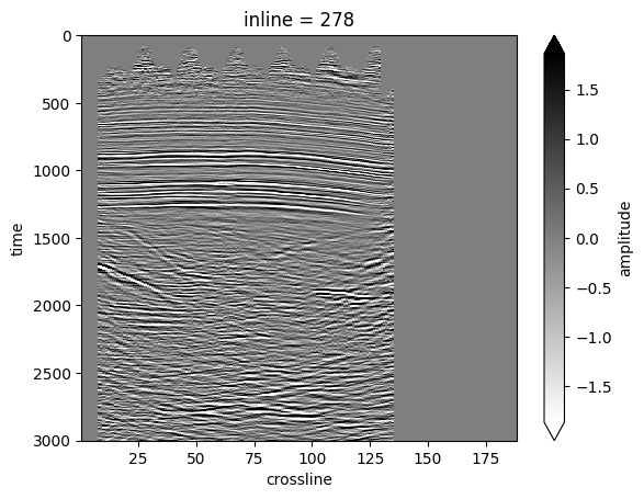
Now we will demonstrate getting an inline from MDIO.

Since MDIO v1 we are using Xarray under the hood, so we can use its convenient indexing. It also handles the plotting with proper dimension coordinate labels.

MDIO stores summary statistics. We can calculate the standard deviation (std) value of the dataset to adjust the gain.

from mdio.builder.schemas.v1.stats import SummaryStatistics

stats = SummaryStatistics.model_validate_json(dataset["amplitude"].attrs["statsV1"])
std = ((stats.sum_squares / stats.count) - (stats.sum / stats.count) ** 2) ** 0.5

il_dataset = dataset.sel(inline=278)
il_amp = il_dataset["amplitude"].T
il_amp.plot(vmin=-2 * std, vmax=2 * std, cmap="gray_r", yincrease=False);

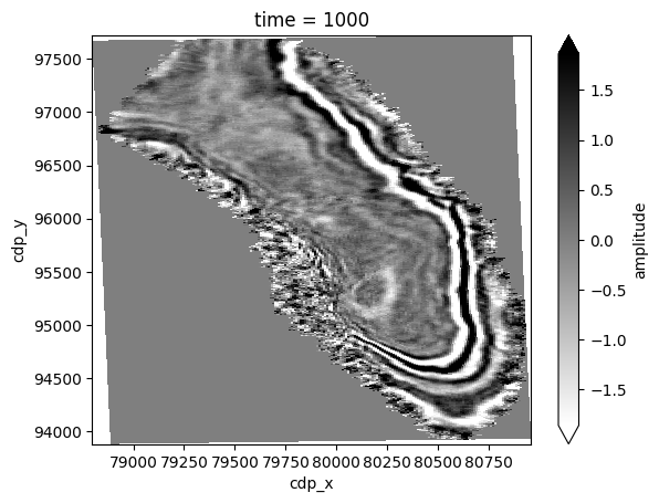
Let’s do the same with a time slice.

We will display two-way-time at 1,000 ms.

Note that since we parse the X/Y coordinates, we can plot time slice in real world coordinates.

twt_data = dataset["amplitude"].sel(time=1000)
twt_data.plot(vmin=-2 * std, vmax=2 * std, cmap="gray_r", x="cdp_x", y="cdp_y");

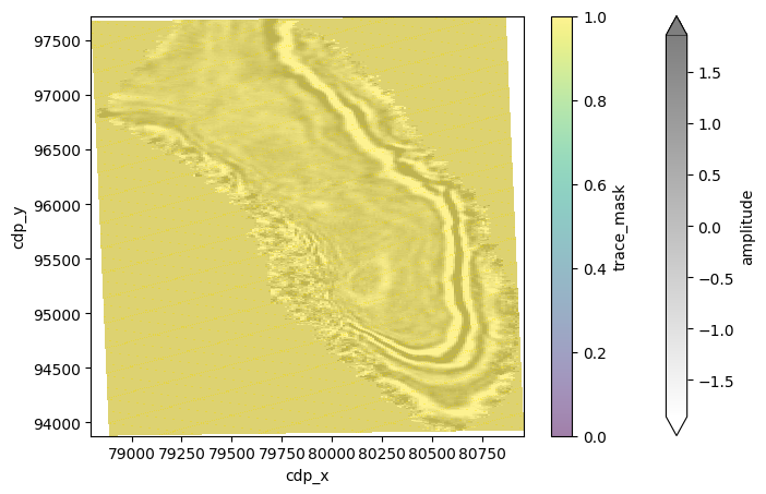
We can also overlay live mask with the time slice. However, in this example, the dataset is zero-padded.

The live trace mask will always show True (yellow).

trace_mask = dataset.trace_mask[:]

twt_data.plot(vmin=-2 * std, vmax=2 * std, cmap="gray_r", x="cdp_x", y="cdp_y", alpha=0.5, figsize=(8, 5))
trace_mask.plot(vmin=0, vmax=1, x="cdp_x", y="cdp_y", alpha=0.5);

Query Headers

We can query headers for the whole dataset very quickly because they are separated from the seismic wavefield.

Let’s get all the headers for X and Y coordinates in this dataset.

Note that the header maps will still share the geometry/grid of the dataset!

The compute property fetches the lazily opened MDIO values.

dataset.headers["cdp_x"].compute()

<xarray.DataArray 'cdp_x' (inline: 345, crossline: 188)> Size: 519kB
array([[78893.7, 78904.7, 78915.7, ..., 80928.2, 80939.2, 80950.2],
       [78893.5, 78904.5, 78915.5, ..., 80927.9, 80938.9, 80949.9],
       [78893.2, 78904.2, 78915.2, ..., 80927.6, 80938.6, 80949.6],
       ...,
       [78804.4, 78815.4, 78826.4, ..., 80838.9, 80849.9, 80860.9],
       [78804.2, 78815.2, 78826.2, ..., 80838.6, 80849.6, 80860.6],
       [78803.9, 78814.9, 78825.9, ..., 80838.3, 80849.3, 80860.3]],
      shape=(345, 188))
Coordinates:
  * inline     (inline) int32 1kB 1 2 3 4 5 6 7 ... 339 340 341 342 343 344 345
  * crossline  (crossline) int32 752B 1 2 3 4 5 6 7 ... 183 184 185 186 187 188
    cdp_y      (inline, crossline) float64 519kB 9.388e+04 ... 9.772e+04
    cdp_x      (inline, crossline) float64 519kB 7.889e+04 ... 8.086e+04
Attributes:
    unitsV1:  {'length': 'ft'}

xarray.DataArray

'cdp_x'

• inline: 345
• crossline: 188

• 7.889e+04 7.89e+04 7.892e+04 ... 8.084e+04 8.085e+04 8.086e+04

  array([[78893.7, 78904.7, 78915.7, ..., 80928.2, 80939.2, 80950.2],
         [78893.5, 78904.5, 78915.5, ..., 80927.9, 80938.9, 80949.9],
         [78893.2, 78904.2, 78915.2, ..., 80927.6, 80938.6, 80949.6],
         ...,
         [78804.4, 78815.4, 78826.4, ..., 80838.9, 80849.9, 80860.9],
         [78804.2, 78815.2, 78826.2, ..., 80838.6, 80849.6, 80860.6],
         [78803.9, 78814.9, 78825.9, ..., 80838.3, 80849.3, 80860.3]],
        shape=(345, 188))

• Coordinates: (4)
  • inline
    (inline)
    int32
    1 2 3 4 5 6 ... 341 342 343 344 345

    array([  1,   2,   3, ..., 343, 344, 345], shape=(345,), dtype=int32)

  • crossline
    (crossline)
    int32
    1 2 3 4 5 6 ... 184 185 186 187 188

    array([  1,   2,   3,   4,   5,   6,   7,   8,   9,  10,  11,  12,  13,  14,
            15,  16,  17,  18,  19,  20,  21,  22,  23,  24,  25,  26,  27,  28,
            29,  30,  31,  32,  33,  34,  35,  36,  37,  38,  39,  40,  41,  42,
            43,  44,  45,  46,  47,  48,  49,  50,  51,  52,  53,  54,  55,  56,
            57,  58,  59,  60,  61,  62,  63,  64,  65,  66,  67,  68,  69,  70,
            71,  72,  73,  74,  75,  76,  77,  78,  79,  80,  81,  82,  83,  84,
            85,  86,  87,  88,  89,  90,  91,  92,  93,  94,  95,  96,  97,  98,
            99, 100, 101, 102, 103, 104, 105, 106, 107, 108, 109, 110, 111, 112,
           113, 114, 115, 116, 117, 118, 119, 120, 121, 122, 123, 124, 125, 126,
           127, 128, 129, 130, 131, 132, 133, 134, 135, 136, 137, 138, 139, 140,
           141, 142, 143, 144, 145, 146, 147, 148, 149, 150, 151, 152, 153, 154,
           155, 156, 157, 158, 159, 160, 161, 162, 163, 164, 165, 166, 167, 168,
           169, 170, 171, 172, 173, 174, 175, 176, 177, 178, 179, 180, 181, 182,
           183, 184, 185, 186, 187, 188], dtype=int32)

  • cdp_y
    (inline, crossline)
    float64
    9.388e+04 9.388e+04 ... 9.772e+04

    unitsV1 :

    {'length': 'ft'}

    array([[93884.6, 93884.8, 93885.1, ..., 93932.9, 93933.1, 93933.4],
           [93895.6, 93895.8, 93896.1, ..., 93943.9, 93944.1, 93944.4],
           [93906.6, 93906.8, 93907.1, ..., 93954.9, 93955.1, 93955.4],
           ...,
           [97645.5, 97645.8, 97646. , ..., 97693.8, 97694.1, 97694.3],
           [97656.5, 97656.8, 97657. , ..., 97704.8, 97705.1, 97705.3],
           [97667.5, 97667.8, 97668. , ..., 97715.8, 97716.1, 97716.3]],
          shape=(345, 188))

  • cdp_x
    (inline, crossline)
    float64
    7.889e+04 7.89e+04 ... 8.086e+04

    unitsV1 :

    {'length': 'ft'}

    array([[78893.7, 78904.7, 78915.7, ..., 80928.2, 80939.2, 80950.2],
           [78893.5, 78904.5, 78915.5, ..., 80927.9, 80938.9, 80949.9],
           [78893.2, 78904.2, 78915.2, ..., 80927.6, 80938.6, 80949.6],
           ...,
           [78804.4, 78815.4, 78826.4, ..., 80838.9, 80849.9, 80860.9],
           [78804.2, 78815.2, 78826.2, ..., 80838.6, 80849.6, 80860.6],
           [78803.9, 78814.9, 78825.9, ..., 80838.3, 80849.3, 80860.3]],
          shape=(345, 188))

• Attributes: (1)

  unitsV1 :

  {'length': 'ft'}

dataset.headers["cdp_y"].compute()

<xarray.DataArray 'cdp_y' (inline: 345, crossline: 188)> Size: 519kB
array([[93884.6, 93884.8, 93885.1, ..., 93932.9, 93933.1, 93933.4],
       [93895.6, 93895.8, 93896.1, ..., 93943.9, 93944.1, 93944.4],
       [93906.6, 93906.8, 93907.1, ..., 93954.9, 93955.1, 93955.4],
       ...,
       [97645.5, 97645.8, 97646. , ..., 97693.8, 97694.1, 97694.3],
       [97656.5, 97656.8, 97657. , ..., 97704.8, 97705.1, 97705.3],
       [97667.5, 97667.8, 97668. , ..., 97715.8, 97716.1, 97716.3]],
      shape=(345, 188))
Coordinates:
  * inline     (inline) int32 1kB 1 2 3 4 5 6 7 ... 339 340 341 342 343 344 345
  * crossline  (crossline) int32 752B 1 2 3 4 5 6 7 ... 183 184 185 186 187 188
    cdp_y      (inline, crossline) float64 519kB 9.388e+04 ... 9.772e+04
    cdp_x      (inline, crossline) float64 519kB 7.889e+04 ... 8.086e+04
Attributes:
    unitsV1:  {'length': 'ft'}

xarray.DataArray

'cdp_y'

• inline: 345
• crossline: 188

• 9.388e+04 9.388e+04 9.389e+04 ... 9.772e+04 9.772e+04 9.772e+04

  array([[93884.6, 93884.8, 93885.1, ..., 93932.9, 93933.1, 93933.4],
         [93895.6, 93895.8, 93896.1, ..., 93943.9, 93944.1, 93944.4],
         [93906.6, 93906.8, 93907.1, ..., 93954.9, 93955.1, 93955.4],
         ...,
         [97645.5, 97645.8, 97646. , ..., 97693.8, 97694.1, 97694.3],
         [97656.5, 97656.8, 97657. , ..., 97704.8, 97705.1, 97705.3],
         [97667.5, 97667.8, 97668. , ..., 97715.8, 97716.1, 97716.3]],
        shape=(345, 188))

• Coordinates: (4)
  • inline
    (inline)
    int32
    1 2 3 4 5 6 ... 341 342 343 344 345

    array([  1,   2,   3, ..., 343, 344, 345], shape=(345,), dtype=int32)

  • crossline
    (crossline)
    int32
    1 2 3 4 5 6 ... 184 185 186 187 188

    array([  1,   2,   3,   4,   5,   6,   7,   8,   9,  10,  11,  12,  13,  14,
            15,  16,  17,  18,  19,  20,  21,  22,  23,  24,  25,  26,  27,  28,
            29,  30,  31,  32,  33,  34,  35,  36,  37,  38,  39,  40,  41,  42,
            43,  44,  45,  46,  47,  48,  49,  50,  51,  52,  53,  54,  55,  56,
            57,  58,  59,  60,  61,  62,  63,  64,  65,  66,  67,  68,  69,  70,
            71,  72,  73,  74,  75,  76,  77,  78,  79,  80,  81,  82,  83,  84,
            85,  86,  87,  88,  89,  90,  91,  92,  93,  94,  95,  96,  97,  98,
            99, 100, 101, 102, 103, 104, 105, 106, 107, 108, 109, 110, 111, 112,
           113, 114, 115, 116, 117, 118, 119, 120, 121, 122, 123, 124, 125, 126,
           127, 128, 129, 130, 131, 132, 133, 134, 135, 136, 137, 138, 139, 140,
           141, 142, 143, 144, 145, 146, 147, 148, 149, 150, 151, 152, 153, 154,
           155, 156, 157, 158, 159, 160, 161, 162, 163, 164, 165, 166, 167, 168,
           169, 170, 171, 172, 173, 174, 175, 176, 177, 178, 179, 180, 181, 182,
           183, 184, 185, 186, 187, 188], dtype=int32)

  • cdp_y
    (inline, crossline)
    float64
    9.388e+04 9.388e+04 ... 9.772e+04

    unitsV1 :

    {'length': 'ft'}

    array([[93884.6, 93884.8, 93885.1, ..., 93932.9, 93933.1, 93933.4],
           [93895.6, 93895.8, 93896.1, ..., 93943.9, 93944.1, 93944.4],
           [93906.6, 93906.8, 93907.1, ..., 93954.9, 93955.1, 93955.4],
           ...,
           [97645.5, 97645.8, 97646. , ..., 97693.8, 97694.1, 97694.3],
           [97656.5, 97656.8, 97657. , ..., 97704.8, 97705.1, 97705.3],
           [97667.5, 97667.8, 97668. , ..., 97715.8, 97716.1, 97716.3]],
          shape=(345, 188))

  • cdp_x
    (inline, crossline)
    float64
    7.889e+04 7.89e+04 ... 8.086e+04

    unitsV1 :

    {'length': 'ft'}

    array([[78893.7, 78904.7, 78915.7, ..., 80928.2, 80939.2, 80950.2],
           [78893.5, 78904.5, 78915.5, ..., 80927.9, 80938.9, 80949.9],
           [78893.2, 78904.2, 78915.2, ..., 80927.6, 80938.6, 80949.6],
           ...,
           [78804.4, 78815.4, 78826.4, ..., 80838.9, 80849.9, 80860.9],
           [78804.2, 78815.2, 78826.2, ..., 80838.6, 80849.6, 80860.6],
           [78803.9, 78814.9, 78825.9, ..., 80838.3, 80849.3, 80860.3]],
          shape=(345, 188))

• Attributes: (1)

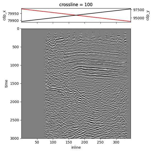
  unitsV1 :

  {'length': 'ft'}

As we mentioned before, we can also get specific dataset slices of headers while fetching a slice.

Let’s fetch a crossline; we are still using some previous parameters.

Since the sliced dataset contains the headers as well, we can plot the headers on top of the image.

Full headers can be mapped and plotted as well, but we won’t demonstrate that here.

xl_dataset = dataset.sel(crossline=100)  # slices everything available in MDIO dataset!

cdp_x_header = xl_dataset["cdp_x"]
cdp_y_header = xl_dataset["cdp_y"]
image = xl_dataset["amplitude"].T

# Build plot from here
gs_kw = {"height_ratios": (1, 8)}
fig, (hdr_ax, img_ax) = plt.subplots(2, 1, figsize=(6, 6), gridspec_kw=gs_kw, sharex="all")
hdr_ax2 = hdr_ax.twinx()

cdp_x_header.plot(ax=hdr_ax, c="red")
cdp_y_header.plot(ax=hdr_ax2, c="black")
image.plot(ax=img_ax, vmin=-2 * std, vmax=2 * std, cmap="gray_r", yincrease=False, add_colorbar=False)
img_ax.set_title("")
hdr_ax.set_xlabel("")

plt.tight_layout()

MDIO to SEG-Y Conversion

Finally, let’s demonstrate going back to SEG-Y.

We will use the convenient mdio_to_segy function and write it out as a round-trip file.

The output spec can be modified if we want to write things to different byte locations, etc, but we will use the same one as before.

from mdio import mdio_to_segy

mdio_to_segy(
    input_path="filt_mig.mdio",
    output_path="filt_mig_roundtrip.sgy",
    segy_spec=teapot_segy_spec,
)

Validate Round-Trip SEG-Y File

We can validate if the round-trip SEG-Y file is matching the original using TGSAI/segy.

Step by step:

• Open original file

• Open round-trip file

• Compare text headers

• Compare binary headers

• Compare 100 random headers and traces

import numpy as np
from segy import SegyFile

original_segy = SegyFile(input_url)
roundtrip_segy = SegyFile("filt_mig_roundtrip.sgy")

# Compare text header
assert original_segy.text_header == roundtrip_segy.text_header

# Compare bin header
assert original_segy.binary_header == roundtrip_segy.binary_header

# Compare 100 random trace headers and traces
rng = np.random.default_rng()
rand_indices = rng.integers(low=0, high=original_segy.num_traces, size=100)
for idx in rand_indices:
    np.testing.assert_equal(original_segy.trace[idx], roundtrip_segy.trace[idx])

print("Files identical!")

Files identical!